Demo Workflow & Analysis Modules

Overview

The rdmpy toolkit provides five integrated analysis modules that work together to examine UK railway delay propagation from multiple perspectives. Each module addresses different analytical questions and levels of network granularity.

The following diagram illustrates how these modules interconnect, from raw data collection through to final analysis outputs:

Demo Specifications

1. Aggregate View

Purpose: Quantify the overall impact of a specific incident across the network.

View the interactive demo notebook on GitHub

Analytical Focus:

• System-level incident impact assessment

• Total delay minutes across all affected stations

• Total cancellations recorded

• Delay severity distribution

Input Parameters:

• Incident code (integer)

• Incident date (string, format: ‘DD-MMM-YYYY’, e.g., ‘24-MAY-2024’)

Output:

• Dictionary containing: - Total delay minutes - Total number of cancellations - Delay severity statistics - Incident duration information

When to Use:

• Quick overview of incident impact magnitude

• Comparing severity across different incidents

• Identifying significant disruption events

• Starting point for deeper investigation

Related Functions:

• aggregate_view() - Single day analysis

• aggregate_view_multiday() - Multi-day incident analysis

Example Usage: Analyze incident 499279 from 24-MAY-2024 to understand total network impact.

result1 = aggregate_view_multiday(499279, "24-MAY-2024")
print("\nSummary:")
if result1:
    for key, value in result1.items():
        print(f"  {key}: {value}")

Aggregate View output: (a) total delay minutes per hour over the 24-hour timeline, (b) delay severity distribution, and (c) individual delay and cancellation events.

—

2. Incident View

Purpose: Detailed spatial and temporal analysis of delay propagation during a specific incident.

View the interactive demo notebook on GitHub

Analytical Focus:

• Temporal progression of delays over time

• Spatial distribution of affected stations

• Granular incident-level delay data

• Network ripple effects and cascading delays

Input Parameters:

• Incident code (integer)

• Incident date (string, format: ‘DD-MMM-YYYY’)

• Analysis date (date to analyze)

• Analysis start time (string, format: ‘HHMM’, e.g., ‘0900’)

• Period duration (integer, minutes to analyze)

• Interval minutes (optional, for heatmap animation, default: 10)

Output:

• Tabular data (pandas DataFrame) of all delays during the analysis period

• Incident start timestamp

• Analysis period definition

Optional Outputs:

• Animated HTML heatmap showing spatial-temporal progression

• Interactive map with delay intensity by location

When to Use:

• Understanding how delays propagate geographically

• Analyzing the ripple effects of a single incident

• Creating visualizations of incident impact over time

• Examining when and where the most severe impacts occurred

• Investigating whether incidents affect specific regions or network-wide

Related Functions:

• incident_view() - Returns tabular delay data

• incident_view_heatmap_html() - Creates animated heat maps

Example Usage: Analyze incident 64326 from 07-DEC-2024, starting at 09:00 for 30 minutes, to see spatial-temporal delay propagation.

# Generate animated network heatmap
incident_code = 62537
incident_date = '07-DEC-2024'
analysis_date = '07-DEC-2024'
analysis_hhmm = '0600'
period_minutes = 1440
interval_minutes = 60

output_file = (
    f'heatmap_incident_{incident_code}'
    f'_{analysis_date.replace("-", "_")}'
    f'_{analysis_hhmm}_period{period_minutes}min'
    f'_interval{interval_minutes}min.html'
)

heatmap_html = incident_view_heatmap_html(
    incident_code=incident_code,
    incident_date=incident_date,
    analysis_date=analysis_date,
    analysis_hhmm=analysis_hhmm,
    period_minutes=period_minutes,
    interval_minutes=interval_minutes,
    output_file=output_file
)

Interactive Output: Incident heatmap for incident 62537 on 07-DEC-2024 (24-hour period, 60-min intervals):

—

3. Time View

Purpose: Network-wide analysis showing aggregate impacts across all incidents on a specific date.

View the interactive demo notebook on GitHub

Analytical Focus:

• Multi-incident day analysis

• Network-wide delay distribution

• Station-level performance on a given date

• Cumulative effects of simultaneous incidents

Input Parameters:

• Analysis date (string, format: ‘DD-MMM-YYYY’, e.g., ‘28-APR-2024’)

• Pre-loaded processed data (all_data from load_processed_data())

Output:

• Interactive HTML map visualization

• Color-coded station markers indicating delay severity

• Network-wide delay aggregation

When to Use:

• Examining specific calendar dates with multiple incidents

• Identifying particularly disruptive days

• Network-level performance assessment

• Understanding cumulative impact when incidents overlap

• Comparing network resilience across different dates

Related Functions:

• create_time_view_html() - Generates interactive network visualization

Example Usage: Visualize network delays on 28-APR-2024 to see the combined impact of all incidents that day.

create_time_view_html('28-APR-2024', all_data)

Interactive Output: Network delay map for 28-APR-2024:

Additional time view examples are available for other dates of interest:

21-OCT-2024 — Talerddig train collision

08-APR-2024 — Storm Kathleen (Day 1)

09-APR-2024 — Storm Kathleen (Day 2)

—

4. Train View

Purpose: Analyze individual train service journeys and reliability metrics.

View the interactive demo notebook on GitHub

Analytical Focus:

• Specific train journey tracking

• Incidents encountered on a particular service

• Train-level delay patterns

• Service reliability statistics

• Route-level performance assessment

Input Parameters:

• Train origin code (STANOX code)

• Train destination code (STANOX code)

• Analysis date (string, format: ‘DD-MMM-YYYY’)

Alternative Parameters (train_view_2 variant):

• Service STANOX (station code)

• Service code (train service identifier)

Output:

• Interactive HTML map showing the complete train journey

• Incidents that affected the specific service

• Delays experienced at each station

• Reliability graphs: - On-time arrival percentage - Delay distribution - Cancellation frequency - Year-based service statistics

When to Use:

• Tracking a specific train service end-to-end

• Understanding why a particular service was delayed

• Assessing service reliability over a year

• Investigating passenger impact on specific routes

• Identifying problematic segments of a route

Related Functions:

• train_view() - Origin/destination based analysis

• train_view_2() - Service code based analysis

• map_train_journey_with_incidents() - Visual journey mapping

• plot_reliability_graphs() - Statistical summaries

Example Usage: Analyze a service from Manchester Piccadilly to London Euston on 21-OCT-2024 to see all incidents encountered and delays at each stop.

result_table = train_view_2(all_data, service_stanox, service_code)
plot_reliability_graphs(all_data, service_stanox, service_code)

Interactive Output: Train journey map for service 21700001 (12931 → 54311, 07-DEC-2024):

Delay distribution per station (overlapping KDEs, capped at 75 min) for service 21700001.

Cumulative delay distribution per station for service 21700001.

—

5. Station View

Purpose: Assess operational performance of a specific railway station under different conditions.

View the interactive demo notebook on GitHub

Analytical Focus:

• Single-station performance assessment

• Comparison of incident vs. normal operations

• Capacity and dwell time analysis

• Delay percentile analysis

• Time-range filtering for targeted analysis

Input Parameters:

• Station ID (STANOX code)

• All processed data (from load_processed_data())

• Number of platforms (integer, default: 6)

• Dwell time in minutes (integer, default: 5)

• Max delay percentile (integer, default: 98)

• Time range (optional, tuple format):

  • time_range=None → Use all available data

  • time_range=('2024-01-15', '2024-01-15') → Single day

  • time_range=('2024-01-01', '2024-06-30') → Date range

  • time_range=('2024-01-15 08:00', '2024-01-15 17:00') → Specific times

Output:

• Comprehensive performance metrics: - Operating characteristics charts - Delay distribution plots - On-time performance statistics - Crowding/capacity assessment

• Separate summaries for: - Incident operation periods - Normal operation periods

When to Use:

• Evaluating how a specific station performs

• Comparing performance during incidents vs. normal operations

• Analyzing seasonal or time-range specific performance

• Identifying peak delay periods at a station

• Understanding platform capacity constraints

• Assessing dwell time impacts

Related Functions:

• station_view() - Full analysis with visualizations

• station_view_yearly() - Yearly interval-based analysis

• station_view_yearly_with_time_range() - Flexible time filtering

• station_analysis_with_time_range() - Detailed comprehensive analysis

Example Usage: Analyze Manchester Piccadilly (station 32000) with 14 platforms for September 2024 to understand performance during a specific month.

comprehensive_results_32000 = station_analysis_with_time_range(
    station_id='32000',
    all_data=all_data,
    num_platforms=14,
    dwell_time_minutes=5,
    max_delay_percentile=98,
    time_range=None  # Full dataset, no time filtering
)

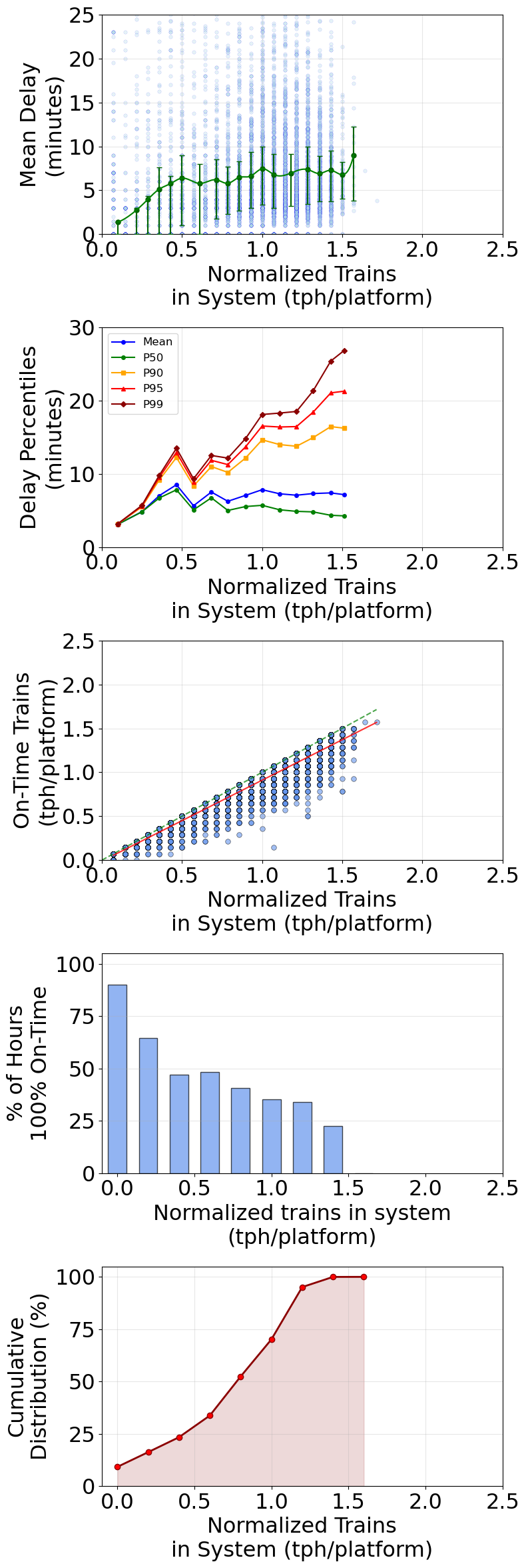
Comprehensive station analysis for Manchester Piccadilly (STANOX 32000): mean delay vs system load, delay percentiles, on-time performance, on-time histogram, and cumulative distribution.

—

Recommended Workflow

For investigating a specific incident:

1. Start with Aggregate View → Get overall impact magnitude

2. Then use Incident View → Understand spatial-temporal propagation

3. Optionally use Train View → See impact on specific services

4. Follow with Station View → Assess individual station responses

For analyzing a particular date:

1. Start with Time View → See network-wide picture

2. Use Station View → Deep-dive into specific stations

3. Use Train View → Track specific services if needed

For station performance assessment:

1. Use Station View → Get comprehensive performance picture

2. Compare with Time View → See how station fits in network context

3. Use Incident View → If specific incidents of interest

For service reliability analysis:

1. Use Train View → Assess overall service performance

2. Use Station View → Examine critical points on the route

3. Use Incident View → Investigate major delays

—

Data Requirements

All demos require pre-processed data from the rdmpy.preprocessor module. Before running any demo, ensure:

1. Raw data has been downloaded from the Rail Data Marketplace

2. Data has been processed using: python -m rdmpy.preprocessor --all-categories

3. Processed data is available in the processed_data/ folder

See Getting Started for data setup instructions.